Generative Adversarial Networks
In this post, we’ll delve deep into Generative Adversarial Networks (GANs) architecture, its loss function and evaluation metrics. We’ll also explore the diverse types of GANs and its alternatives that have been pushing the boundaries of what’s possible in AI.
We're going to dive pretty deep into the rabbit hole, and having a good understanding of machine learning and deep learning is a must for this blog. But if you think you're ready for it 😇, grab a cup of coffee and get ready to dive in deep, because this blog is on GANs. My name is Rahul, and Welcome to TechTalk Verse! 🤟
Overview
Models in machine learning can be classified into two broad categories, i.e., discriminative models (ex. linear regression, neural networks, etc.) and generative models (ex. GANs, VAEs, diffusion etc.). Discriminative models distinguish between classes. Generative models learn to produce realistic examples.
Discriminative models take features as input and output class labels, while generative models take noise and class labels as input and output features. Genearative models take noise as input for stochasticity so that they don’t generate the same thing each time.
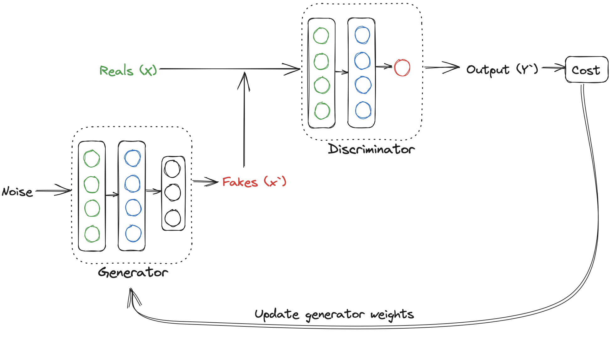
A GAN consists of two models: a generator and a discriminator.
- Discriminator : It learns the probability of class labels (real or fake) given input features. The probabilities are feedback for the generator.
- Generator : It learns the probability of features. It takes noise as input and label (if generating multi-label images).
Loss functions in GANs are called adversarial loss, as the discriminator tries to minimize the loss while the generator tries to maximize it. GANs are trained in an alternative fashion. And the two models i.e., generator and discriminator should always be a similar skill level. This will prevent GANs from getting stuck in a local minima.
Adversarial Loss
Loss functions in GANs are called adversarial loss, as the discriminator tries to minimize the loss while the generator tries to maximize it. Given below are some adversarial losses used in GANs.
BCE Loss
Binary Cross Entropy (BCE) loss is traditionally used for training GANs but its not the best way to do it. BCE loss for GANs is \( \min\limits_{d}\max\limits_{g}J(\theta) \), where, g is generator, d is discriminator and
\( J(\theta) = -\frac{1}{m}\sum\limits_{i=1}^{m}[y^{i}log(h(x^{i},\theta)) + (1-y^{i})log(1-h(x^{i},\theta))] \)
BCE adversarial loss can also be written as :
\( \min\limits_{d}\max\limits_{g}-[E(log(d(x))) + E(1-log(d(g(z))))] \)
Problems with BCE loss
- When discriminator improves too much, the function approximated by BCE loss will contain flat regions and flat regions on the cost functions means vanishing gradients. So, the GANs don’t learn any further.
- Mode collapse happens when generation get stuck in one mode. It happens because discriminator send strong feedback for fake images for particular classes (modes) then generator produces only those classes where discriminator will give green flag.
MSE Loss
- It is Mean Square Error or Least Square loss.
- It helps with vanishing gradients and mode collapse.
- It is more stable than BCE loss, since the gradient is only flat when prediction is exactly correct.
- This loss is used as main adversarial loss in CycleGANs.
\( MSE \ Loss = E_x [ (D(x) - 1)^2] + E_z [ (D(G(z)) - 0)^2] \)
Here, D is discriminator, G is generator, x is for real image and z is for fake images.
Wasserstein Loss
W-loss or Wasserstein Loss approximates Earth Mover’s Distance (EMD). EMD is the effort to make the generated distribution equal to the real distribution.
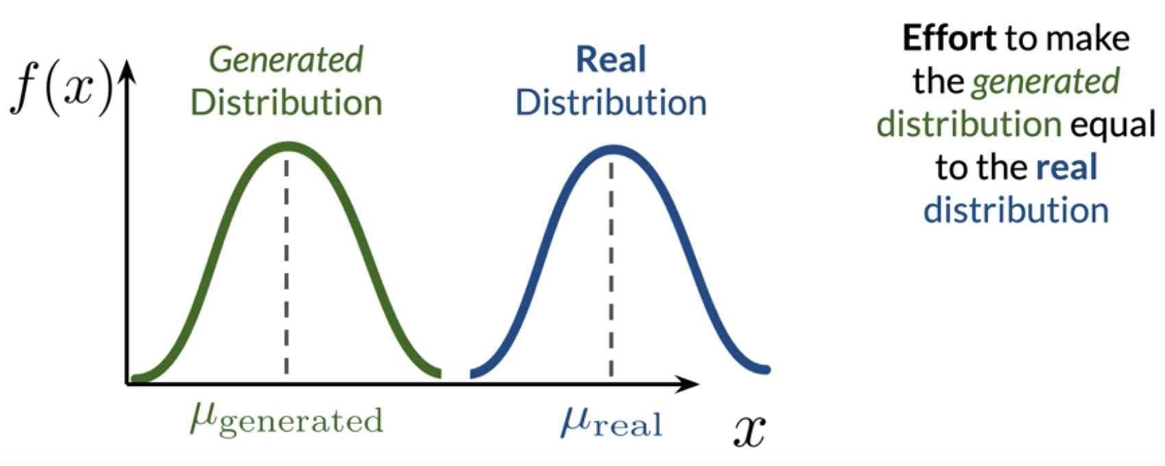
Earth Mover's Distance
\( \min\limits_{d}\max\limits_{g}E(c(x)) - E(c(g(z))) \), where,
g = generator –> minimize distance
c = critic –> maximize distance
Since, EMD doesn't have flat regions when the distributions are very different. So W-loss prevents mode collapse and vanishing gradients problems.
Condition on Wasserstein Critic : It needs to be 1-lipschitz continuous i.e., the norm of the gradient should be at most 1 for every point.
1-lipschitz Continuity Enforcemetn : There are two ways it can be enforced.
Weight Clipping: There is problem with this approach as it limits the learning ability of the critic.Gradinet Penalty: This approach is better as compared the weight clipping as it allows the critic to learn the weights on its own.
SO, W-loss with gradient penalty is given as :
\( \min\limits_{d}\max\limits_{g}E(c(x)) - E(c(g(z))) + \lambda E(|| \Delta C(\hat{x}) ||_{2} - 1)^2 \)
Pixel Distance Loss
This loss term calculates the difference between the fake and real target outputs. Pixel Distance loss term is used in image to image translation models like Pix2Pix. Also, this loss is used with some weights assigned to it along with other losses like BCE loss or W-loss.
\( Pixel \ Distance \ Loss = \sum\limits_{i=1}^{n}| generated \ output - real \ output | \)
GANs Evaluation
As we don’t have ground truth for the generator’s output, its challenging to evaluate GANs. In the case of classifiers, we have labels, but in GANs, we don’t know if its real or fake.
Discriminator models can't be used for evaluation as they overfit the generator they are trained on. And so there is no universal gold-standard discriminator. Fidelity measures image quality and diversity measures variety. Following are some of the evaluation techniques for GANs.
Frechet Inception Distance
For calcualating Frechet Inception Distance (FID), first embeddings for real and fake images are extracted from inception network . These real and fake embeddings are two multivaraiate normal distributions. FID is then calculated with the following formulae:
\( FID = || \mu_x - \mu_y ||^{2} + Tr(\sum x + \sum y - 2 \sqrt{\sum x \sum y}) \)
Shortcomings of FID
- Uses pretrained inception model for embeddings, which may not capture all features.
- Limited statistics used i.e., only mean and covariance.
- Sample size needs to be large for FID to work well.
- Slow to run.
Inception Score
FID uses intermediate features form the Inception-V3 network, while Inception Score (IS) uses the classifications directly. Formulae for IS score is:
\( IS = \exp(E_{x \sim p_g} D_{KL}(p(y|x) || p(y))) \)
Here, KL Divergence i.e., \(D_{KL}(p(y|x) || p(y)) = p(y|x)\log(\frac{p(y|x)}{p(y)}) \)
Shortcomings of IS
- Can be exploited (generate one realistic image of each class)
- Only looks at fake images (no comparison to real images)
- Can miss useful fatures (imagenet isn’t everything)
- It is worse than FID.
HYPE
HYPE i.e., Human Eye Perceptual Evaluation for generative models. In this case human is made use for evaluation. \( HYPE_{time} \) measures time-limited perceptual thresholds where a human is show both real and fake images for certain time interval. \( HYPE_{\infty} \) measures error rate on a percentage of images.
Conditional GANs
Conditional GANs are the GANs where we want to control the class labels of the output images. So, in Conditional GANs, input is noise vector and class vector. Training data needs to be labeled in this case.
Patch GANs
The only difference between a normal GAN and a Patch GAN is that a Patch GAN’s discriminator outputs a matrix of values whose values lies between 0 and 1. These matrix of values give more information about the fakness/realism of generator’s output image for each patch. And the generator also learn about the degree of realism in each part of its generated images. And hence the generator learns better in these GANs.
Style GANs
Style GANs focus on the following things:
- Greater fidelity (quality) on high resolution images.
- Increased diversity of inputs.
- More control over image features.
Following are the major components of StyleGAN:
- Progressive Growing
- Noise Mapping Network
- Adaptive Instance Normalization (AdaIN)
- Style Mixing
- Stochastic Noise
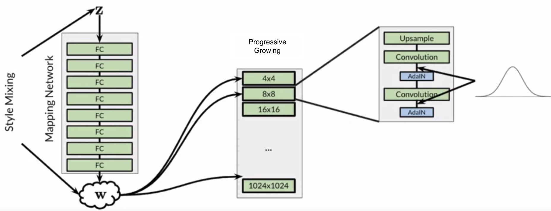
StyleGAN Architecture
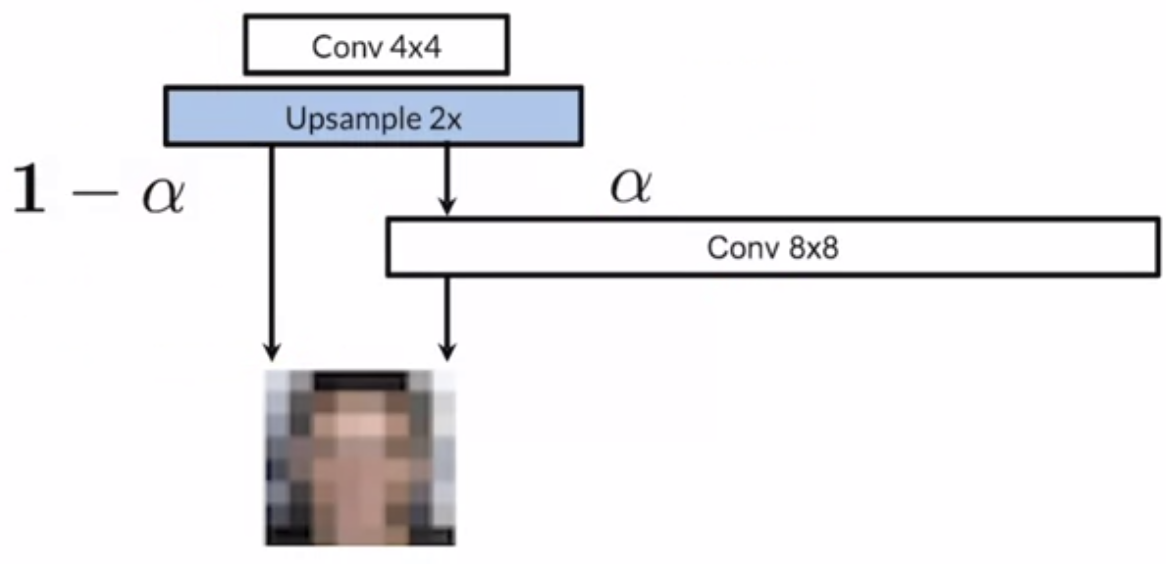
Progressive Growing
Progressive growing means gradually train the generator by increasing the resolution of images being generated in iterations. It helps with faster and more stable training for higher resolutions.
Progressive Growing : Generator
Noise Mapping Network
This is a Multi Layer Perceptron (MLP) network where input in Z space (noise vector) and output is W space (intermediate noise vector). It allows intermediate vector (W) to be in a more disentangled space. And it makes easier to learn 1:1 mappings. It learns linear factors of variations and increase control over features in a more disentangled space. The intermediate noise vector is input to the generator.
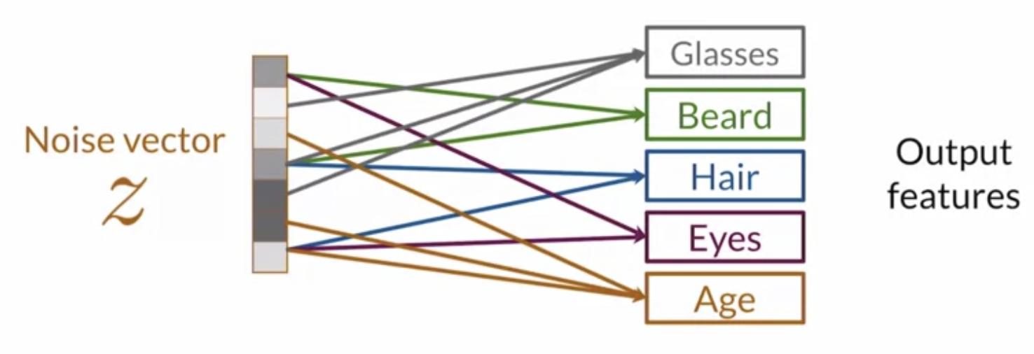
Entangled Z-Space
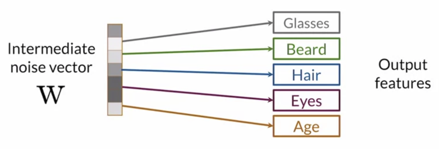
Disentangled W-Space
AdaIN
AdaIN transfers style information onto the generated image from the intermediate noise vector (W). Instance Normalization is used to normalize individual examples before applying style statistics from W. Instance Normalization is similar to batch normalization but instead of taking mean and standard deviation of batch input, it takes mean and standard deviation for just a single whole set of image.
\( AdaIN(x_i,y) = y_{s,i} . \frac{x_i - \mu (x_i)}{\sigma (x_i)} + y_{b,i} \)
Here,
\( i = i^{th} \ instance \)
\( y_{s,i} = scale \ factor \)
\( y_{b,i} = bias \ term \)
Style Mixing
Style means passing two or more noise vectors within the same network in the same time. Style mixing increases diversity that the model sees during training.
Stochastic Noise
Stochastic Noise causes small variation to the output. Coarse or fineness depends where in the network style or noise is added.
- When noise is added in the earlier part of the network, it causes coarser variation.
- When noise is added in the later part of the network, it causes finer variation.
Pix2Pix
Pix2Pix is a famous GAN for paired image to image translation. Pix2Pix is similar to conditional GAN. Following are the details for Pix2Pix architechture
- It takes original image (segmentation map), instead of class vector as input.
- No explicit noise as input is fed. (even if explicit noise was used, it didn’t make any difference).
- Stochasticity is handled during training via dropout.
- Generator is upgraded to UNet model.
- Discriminator is upgraded to Patch GAN.
- \( Loss = BCE \ Loss + \lambda (Pixel \ Distance \ Loss) \)
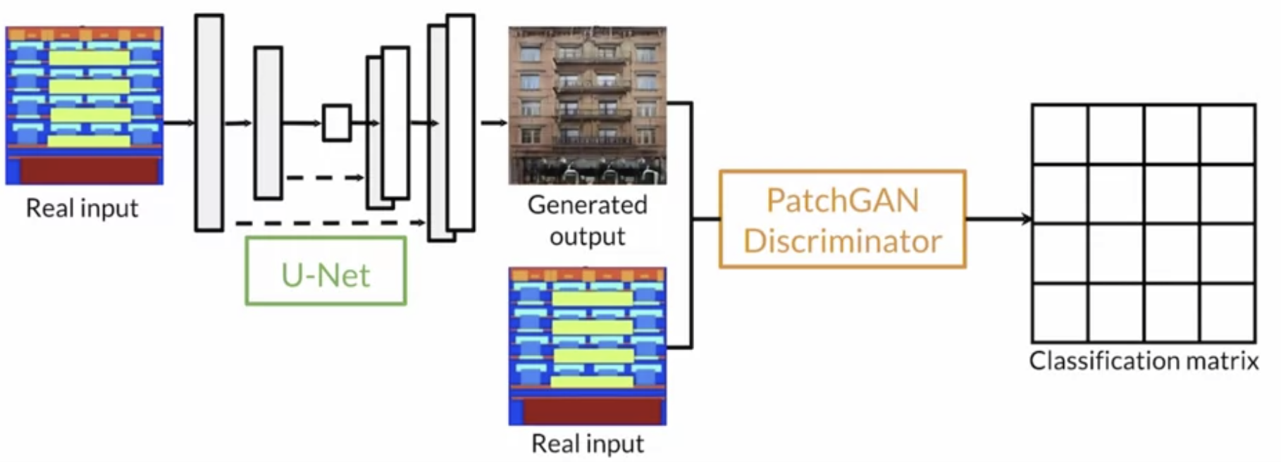
Pix2Pix Architechture
Pix2PixHD and GauGAN are successors of Pix2Pix.
Cycle GANs
Cycle GANs are composed of 2 GANs for unpaired image to image translation. It learns a mapping between two piles of images. It examines common elements of the tow piles (content) and unique elements of each pile (style).
-
Unlike paired image-to-image translation, it is unsupervised.
-
The discriminators are Patch GANs.
-
The generators are similar to a U-Net and DCGAN with additional skip connections.
-
The inputs to the generators and discriminators are similar to Pix2Pix, except :
- There are no real target outputs.
- Each discriminator is in charge of one pile of images.
-
Following Loss terms are present in Cycle GANs
- Mean Square Error (MSE) Loss is used as main adversarial loss.
- Identity Loss is optionally added in CycelGANs to help with color preservation.
- Cycel Consistency Loss helps transfering uncommon style elements between the two GANs, while maintaining common content.
-
Discriminator loss is simple MSE adversarial loss using PatchGANs.
-
Generator has 6 loss terms, 2 from each
- MSE Loss
- Identity Loss
- Cycle Consistency Loss
Data Augmentation
GANs are also used for creating additional data for training. Pros for data augmentation with the help of GANs are :
- Can be better than hand-crafted synthetic examples.
- Can generate more labeled examples.
- Can improve a downstream model’s generalization.
Cons for data augmentation with the help of GANs are :
- Can be limited by the available data in diversity.
- Can overfit to the real training data.
GANs Alternatives
There are some cons for GANs model like unstable training, lack of intrinsic evaluation metrics, no density evaluation. Also, inverting is not straight forward. GANs alternative includes:
- Variational Auto Encoders (VAEs) : Maximize variational lower bound.
- Auto Regressive Models : Relies on previous pixels to generate next pixel.
- Flow Models : Uses invertible mappings for distributions.
- Diffusion Models : Gradually add gaussian noise and then reverse.
VAEs
VAEs are autoencoder model used for generating images, detecting anomalies and removing noise. After the training is done, encoder is looped off (like discriminator in case of GANs), and decoder is used like generator to generate images.
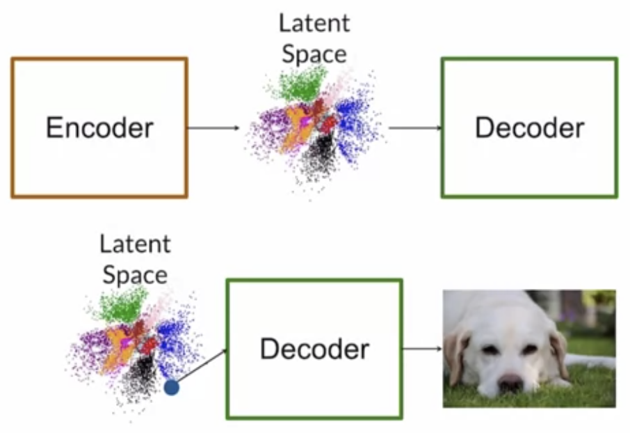
There are advantages of of VAEs like stable training, invertible and have density estimation. However the quality of generated images are low.
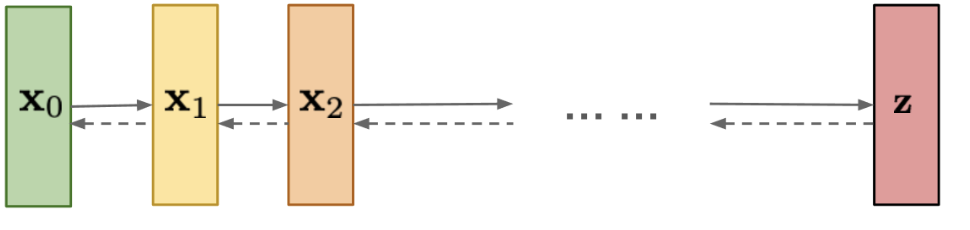
Diffusion Models
Diffusion Models are currently state-of-the-art for generating high quality images. Diffusion models are trained in iterations where, in each successive iteration, gaussian noise is added, and the model has to learn to recover the data by reversing the noising process. After the training, the model is used to generate images by simply passing sample noise.
Diffusion Model Architechture
References
- Coursera GANs Specialization
- Deep Learning by Ian Goodfellow