Reinforcement Learning : Tabular Solution Methods
Multi-armed Bandits
The multi-armed bandit problem serves as an introductory concept in reinforcement learning, much like how the house pricing problem acts as a starting point in machine learning. In the K-armed bandit problem, an agent is presented with a set of ‘k’ actions to choose from, and the agent’s decision results in a corresponding reward. Value of an action is the expected or mean reward given when that action is selected. If we knew the value of each action, then it would be trivial to solve the k-armed bandit problem. So, for solving the multi-armed bandit problem we use sample average method to estimate the action values. $$ q_*(a) \overset{.}{=} E[R_t | A_t=a] $$ $$ Q_t(a) \overset{.}{=} \frac{Sum\ of\ rewards\ when\ a\ taken\ prior\ to\ t}{No.\ of\ times\ a\ taken\ prior\ to\ t} = \frac{\sum_{i=1}^{t-1} R_i }{t-1} $$
Now that we have the action values, we need to select one of the action given the action values. The simplest action selection rule is to select one of the actions with the highest estimated value called greedy action selection method.
$$ A_t \overset{.}{=} \underset{a}{\text{argmax}}Q_t(a) $$
dfdfGreedy action selection always exploits current knowledge to maximize immediate reward. A simple alternative is to behave greedily most of the time, but every once in a while, say with small probability ε, instead select randomly from among all the actions with equal probability, independently of the action-value estimates. We call methods using this near-greedy action selection rule ε-greedy methods. In this way, reward is lower in the short run, during exploration, but higher in the long run because after you have discovered the better actions, you can exploit them many times.
Action values can be calculated incrementally using sample average method as follows :
$$ Q_{n+1} \overset{.}{=} Q_n + \frac{1}{n}(R_n - Q_n) $$
NewEstimate ← OldEstimate + StepSize [Target - OldEstimate].
Step Size is α or 1/n.
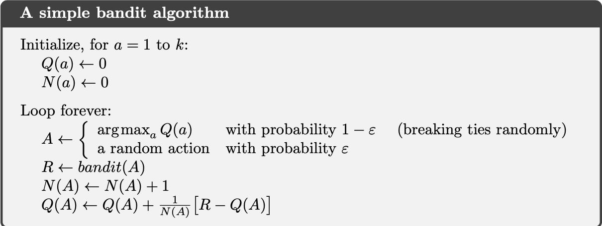
Pseudocode for a complete bandit algorithm
Dynamic Programming
The term dynamic programming (DP) refers to a collection of algorithms that can be used to compute optimal policies given a perfect model of the environment as a Markov decision process (MDP). DP algorithms are obtained by turning Bellman equations into assignments, that is, into update rules for improving approximations of the desired value functions. $$ V_\pi(s) \overset{.}{=} \sum\limits_a \pi(a|s)\sum\limits_{s’,r} p(s’,r|s,a)\left [r + \gamma V_{\pi}(s’) \right ] $$ $$ V_{k+1}(s) \leftarrow \sum\limits_a \pi(a|s)\sum\limits_{s’,r} p(s’,r|s,a)\left [r + \gamma V_{\pi}(s’) \right ] $$
Linear programming methods can also be used to solve MDPs. But linear programming methods become impractical at a much smaller number of states than do DP methods.
Monte Carlo Methods
Monte Carlo is an estimation method that relies on repeated random sampling. Monte Carlo methods estimate values by averaging over a large number of random samples. Monte Carlo methods require only experience - sample sequences of states, actions, and rewards from actual or simulated interaction with an environment. This method is applicable only for episodic tasks. Monte Carlo methods can thus be incremental in an episode-by-episode sense, but not in a step-by-step (online) sense. Monte Carlo methods sample and average returns for each state–action pair much like the bandit methods sample and average rewards for each action. The only difference is in bandit only one state is there while in monte carlo there are multiple states. Monte Carlo update is given as : $$ V(S_t) \leftarrow V(S_t) + \alpha (G_t -V(S_t)) $$
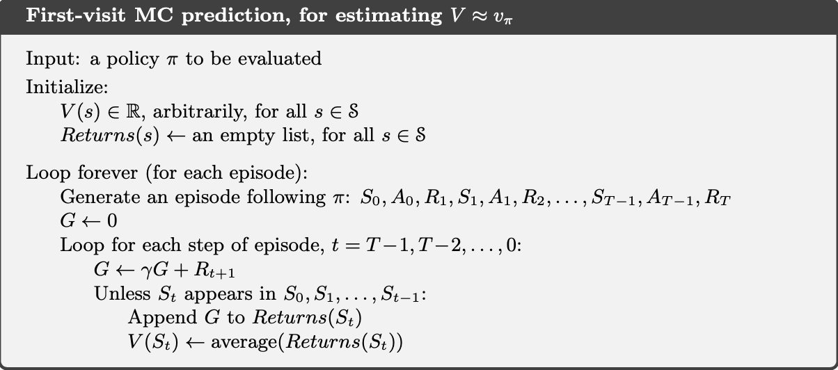
Monte Carlo Value Iteration

Monte Carlo Policy Iteration
There are two learning control methods : on-policy and off-policy methods. The distinguishing feature of on-policy methods is that they estimate the value of a policy while using it for control. In off-policy methods these two functions are separated. In on-policy methods we improve and evaluate the same policy which is being used of selecting the actions. In off-policy methods we improve and evaluate different policy from the one used for selecting actions.
Temporal-Difference Learning
TD learning is a combination of Monte Carlo ideas and dynamic programming (DP) ideas. Like Monte Carlo methods, TD methods can learn directly from raw experience without a model of the environment’s dynamics. Like DP, TD methods update estimates based in part on other learned estimates, without waiting for a final outcome (they bootstrap). Whereas Monte Carlo methods must wait until the end of the episode to determine the increment to V (St) (only then is Gt known), TD methods need to wait only until the next time step.
Temporal-Difference Learning Update is written as :
$$
V(S_t) \leftarrow V(S_t) + \alpha \left[ R_{t+1} + \gamma V(S_{t+1}) -V(S_t) \right]
$$
The target for the Monte Carlo update is Gt, whereas the target for the TD update is R + γV(s) which is also called TD error. This TD method is called TD(0), or one-step TD, because it is a special case of the TD(λ) and n-step TD methods.
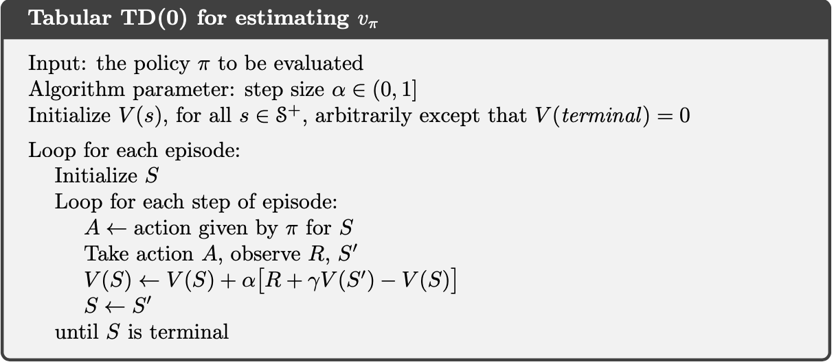
TD(0) : One Step Temporal Difference
SARSA: On-policy TD Control
It is an on-policy algorithm. The agent bootstraps off the value of action its going to take next which is sampled from its behaviour policy. Action selection policy in SARSA is ε-greedy. SARSA Learning Update is written as : $$ Q(S_t, A_t) \leftarrow Q(S_t, A_t) + \alpha \left[ R_{t+1} + \gamma Q(S_{t+1}, A_{t+1}) -Q(S_t, A_t) \right] $$
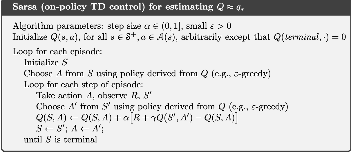
SARSA
Q-learning : Off-policy TD Control
It is off-policy as in Q-learning we bootstrap off the largest action value in the next state.
Q-learning Update is written as :
$$
Q(S_t, A_t) \leftarrow Q(S_t, A_t) + \alpha \left[ R_{t+1} + \gamma\underset{a}{max} Q(S_{t+1}, a) -Q(S_t, A_t) \right ]
$$

Q-learning
Expected SARSA : Off-policy TD Control
It is just like Q-learning except that instead of the maximum over next state–action pairs it uses the expected value, taking into account how likely each action is under the current policy.
Expected SARSA Learning Update is written as :
$$
Q(S_t, A_t) \leftarrow Q(S_t, A_t) + \alpha \left[ R_{t+1} + \gamma E_{\pi}\left [ Q(S_{t+1}, A_{t+1})\ |\ S_{t+1}\right ] -Q(S_t, A_t) \right]
$$
$$
Q(S_t, A_t) \leftarrow Q(S_t, A_t) + \alpha \left[ R_{t+1} + \gamma \sum\limits_a \pi(a|S_{t+1})Q(S_{t+1},a) -Q(S_t, A_t) \right]
$$
References
- Machine Learning: A multistrategy approach by Tom M. Mitchell
- Reinforcement Learning : An Introduction by Andrew Barto and Richard S. Sutton