Reinforcement Learning : Fundamentals

Reinforcement learning is the process of discovering what to do in order to maximise a numerical reward signal. A reinforcement learning system’s primary sub-components are policy, reward signal, value function, agent, and environment.
A policy is a mapping between perceived environmental states and the actions to be taken when those states are present. The objective of a reinforcement learning issue is specified by a reward signal. Value of a state is the total amount of reward an agent can expect to accumulate over the future, starting from that state.
Overview
We seek actions that bring about states of highest value, not highest reward. A state might always yield a low immediate reward but still have a high value because it is regularly followed by other states that yield high rewards. The learner and decision maker is called the agent and every thing else is environment. The agent exists in an environment described by some set of possible states S (shown in the above figure). It can perform any of a set of possible actions A . Each time it performs an action a, in some state s the agent receives a real-valued reward r , that indicates the immediate value of this state-action transition. This produces a sequence of states s, actions a, and immediate rewards r as shown in the figure. The agent’s task is to learn a control policy, 𝝅 : S → A, that outputs an appropriate action a from the set A , given the current state s from the set S. It does so by maximizing the expected sum of these rewards, with future rewards discounted exponentially by their delay. The problem of learning a control policy to choose actions is similar in some respects to the function approximation problems. However, reinforcement learning problem differs from other function approximation tasks in several important respects which includes delayed rewards, exploration, partially observable states and life-long learning.
Multi-armed Bandits
The multi-armed bandit problem serves as an introductory concept in reinforcement learning, much like how the house pricing problem acts as a starting point in machine learning. In the K-armed bandit problem, an agent is presented with a set of ‘k’ actions to choose from, and the agent’s decision results in a corresponding reward. Value of an action is the expected or mean reward given when that action is selected. If we knew the value of each action, then it would be trivial to solve the k-armed bandit problem. So, for solving the multi-armed bandit problem we use sample average method to estimate the action values. $$ q_*(a) \overset{.}{=} E[R_t | A_t=a] $$ $$ Q_t(a) \overset{.}{=} \frac{Sum\ of\ rewards\ when\ a\ taken\ prior\ to\ t}{No.\ of\ times\ a\ taken\ prior\ to\ t} = \frac{\sum_{i=1}^{t-1} R_i }{t-1} $$
Now that we have the action values, we need to select one of the action given the action values. The simplest action selection rule is to select one of the actions with the highest estimated value called greedy action selection method.
$$ A_t \overset{.}{=} \underset{a}{\text{argmax}}Q_t(a) $$
Greedy action selection always exploits current knowledge to maximize immediate reward. A simple alternative is to behave greedily most of the time, but every once in a while, say with small probability ε, instead select randomly from among all the actions with equal probability, independently of the action-value estimates. We call methods using this near-greedy action selection rule ε-greedy methods. In this way, reward is lower in the short run, during exploration, but higher in the long run because after you have discovered the better actions, you can exploit them many times.
Action values can be calculated incrementally using sample average method as follows :
$$ Q_{n+1} \overset{.}{=} Q_n + \frac{1}{n}(R_n - Q_n) $$
NewEstimate ← OldEstimate + StepSize [Target - OldEstimate].
Step Size is α or 1/n.
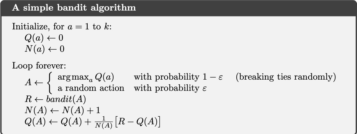
Bandit algorithm using incrementally computed sample averages and ε-greedy action selection
Markov Decision Process (MDP)
MDPs provide general framework for sequential decision making. The dynamics of a MDP are defined by probability distribution. MDPs have one assumption called markov property i.e., the present state contains all the information necessary to predict the future. The present state is sufficient and remembering earlier states would not improve prediction about future.
Whereas in bandit problems we estimated the value of each action a, in MDPs we estimate the value of each action a in each state s.
Here, p specifies a probability distribution for each choice of s and a, that is, :
$$
\sum\limits_{s’ \epsilon S}\sum\limits_{r \epsilon R}p(s’,r|s,a) = 1, for\ all\ s\ \epsilon S, a \epsilon A(s)
$$
Returns and Episodes
Return is simply the sum of rewards which the agent get after each action. $$ G_t \overset{.}{=} R_{t+1} + R_{t+2} + R_{t+3} + . . . . + R_{T} $$ When the agent–environment interaction breaks naturally into subsequences, which we call episodes. Each episode ends in a terminal state. In many cases the agent–environment interaction does not break naturally into identifiable episodes, but goes on continually without limit which is called continuing tasks. The return formulation is problematic for continuing tasks as return would become infinity. So, the agent tries to select actions so that the sum of the discounted rewards it receives over the future is maximized. So discounted return is defined as : $$ G_t \overset{.}{=} R_{t+1} + \gamma R_{t+2} + \gamma^2 R_{t+3} + . . . . = \sum\limits_{k=0}^{\infty}\gamma^k R_{t+k+1} $$
$$ G_t \overset{.}{=} R_{t+1} + \gamma G_{t+1} $$
Value Functions
State value functions represent the expected return from a given state under a specified policy. Action value functions represent the expected return from a given state after taking a specific action and following a specified policy.
State-value function for policy π :
$$
V_\pi(s) \overset{.}{=} E_\pi\left [ G_t|S_{t}=s \right ] = E_\pi\left [\sum\limits_{k=0}^{\infty}\gamma^k R_{t+k+1}|S_{t}=s \right ], for\ all\ s\ \epsilon\ S
$$
Action-value function for policy π:
$$
q_\pi(s,a) \overset{.}{=} E_\pi\left [ G_t|S_{t}=s, A_t=a \right ] = E_\pi\left [\sum\limits_{k=0}^{\infty}\gamma^k R_{t+k+1}|S_{t}=s, A_t = a \right ]
$$
The subscript 兀 indicates the value function is contingent on the agent selecting actions according to Pi. And the subscirpt 兀 on expectation indicates that the expectation is computed with respect to policy pi.
Bellman Equation
Bellman equation allows us to relate value of current state to the value of future states without waiting to observe all the future rewards. It formalizes the connection between the current state and its possible successors. $$ V_\pi(s) \overset{.}{=} E_\pi\left [ G_t|S_{t}=s \right ] $$ $$ V_\pi(s) \overset{.}{=} E_\pi\left [ R_{t+1} + \gamma G_{t+1} |S_{t}=s \right ] $$ $$ V_\pi(s) \overset{.}{=} \sum\limits_a \pi(a|s)\sum\limits_{s’}\sum\limits_r p(s’,r|s,a)\left [r + \gamma E_{\pi}\left [ G_{t+1}|S_{t+1}=s’ \right ] \right ] $$ $$ V_\pi(s) \overset{.}{=} \sum\limits_a \pi(a|s)\sum\limits_{s’,r} p(s’,r|s,a)\left [r + \gamma V_{\pi}(s’) \right ], for\ all\ s\ \epsilon\ S $$
Policy Iteration
Policy Iteration = Policy Evaluation + Policy Improvement
Policy evaluation is the task of determining the value function for a specific policy.
Policy Control or Policy Improvement is the task of finding a policy which maximizes the value function.
In policy iteration, these two processes alternate, each completing before the other begins. In value iteration only a single iteration of policy evaluation is performed in between each policy improvement.
An optimal policy is defined as the policy with highest possible value function in all states.
References
- Machine Learning: A multistrategy approach by Tom M. Mitchell
- Reinforcement Learning : An Introduction by Andrew Barto and Richard S. Sutton