LLM Inferencing Basics

LLM inference is an iterative process, where each new forward pass of the model generates one additional completion token. The initial ingestion (prefill) of the prompt takes as much time as generating each subsequent token. During the prefill phase, the model pre-computes certain inputs of the attention mechanism, specifically the key (k) and value (v) matrices, which remain constant for the remainder of the inference process.
LLMs inferencing costs way more than its training. One might think that by optimizing model training and its architecture, its inferencing will also be optimal. But this is not the case. LLMs generates there output iteratively and most of the time it is memory bound and not compute bound because it takes more time to to load 1MB of data to the GPU’s compute cores than it does for those compute cores to perform computation on 1MB of data. In this post, I’ve discussed various inference optimization techniques, such as KV cache, batching strategies, paged attention, model parallelism, and quantization.
We're going to dive pretty deep into the rabbit hole, and having a good understanding of machine learning and deep learning is a must for this blog. But if you think you're ready for it 😇, grab a cup of coffee and get ready to dive in deep, because this blog is on LLM Inferencing. My name is Rahul, and Welcome to TechTalk Verse! 🤟
Basics
Parameters Calculation
First let’s calculate apporoximate numbers of parameters in an LLM architecture. Consider \( n_{l} \) as number of decoder layers and each decoder layer consists of self attention layer and a feed forward network. \( d_{model} \) is the token embedding dimention. \( n_{heads} \) is number of heads and \( d_{head} \) is dimention of each head. Now, weights per layer consists of following :
- \( W_{q}, W_{k}, W_{v} \) i.e., key, query and value matrices. And each matrix is of size \( d_{model}*n_{heads}*d_{head} \).
- \( W_{o} \) matrix which is used on the output of self-attention layer and before feed forward layer. \( W_{o} \) matrix is also of size \( d_{model}*n_{heads}*d_{head} \).
- Feed Forward Network consists of 2 layers and each of size \( {d_{model}}^{2}*4 \) .
Also, in most of the tranformer architecture, \( d_{model} = n_{heads}*d_{head} \). So, number of parameters in a typical LLM block
=> \( 4*d_{model}*n_{heads}*d_{head} \) (K, Q, V, \( W_{o} \) matrices) + \( 4*2*{d_{model}}^{2} \) (feed forward layers).
=> No. of parameters, P = \( 12*n_{layers}*{d_{model}}^{2} \)
In the above calculation, most of the parameters have been accounted. But there are some more parameters which includes the following :
- token embeddings : \( 2*n_{tokens}*d_{model} \)
- positional embeddings : \( n_{sequence}*d_{model} \)
- layernorm : \( d_{model} \)
- biases
KV Cache Calculation
When you’re doing auto-regressive text generation, you predict one token at a time. When predicting a given token, in the attention layer, you need to compute the attention between the most recent token and all tokens generated so far – you use the query from the last token, but the key and the value from all tokens generated so far. This means you have no benefit in caching the query, but you save a few computations if you cache the key and the value.
Per token, number of bytes we store for kv cache = \( 2*2*n_{layers}*n_{heads}*d_{heads} \) = \( 4*n_{layers}*n_{heads}*d_{heads} \)
Here, the first factor of 2 is for two vectors, k and v. And the second 2 is for number of bytes (assuming fp16).
Compute vs Memory
Inference is memory bandwidth bound. Despite having high flops, LLMs struggle to achieve saturation because of chip’s memory bandwidth is spent on loading model parameters. For a model to output one token, every parameter must be sent from the memory to the compute cores to perform the forward pass inference calculation. A 7B parameter model is 14GB of data (fp16). Thus to generate 1000 tokens/s requires 14 TB/sec of memory bandwidth.
Minimal Batch Size to avoid wasting flops = \( B^* \) = (FLOPS)/(Memory Bandwidth)
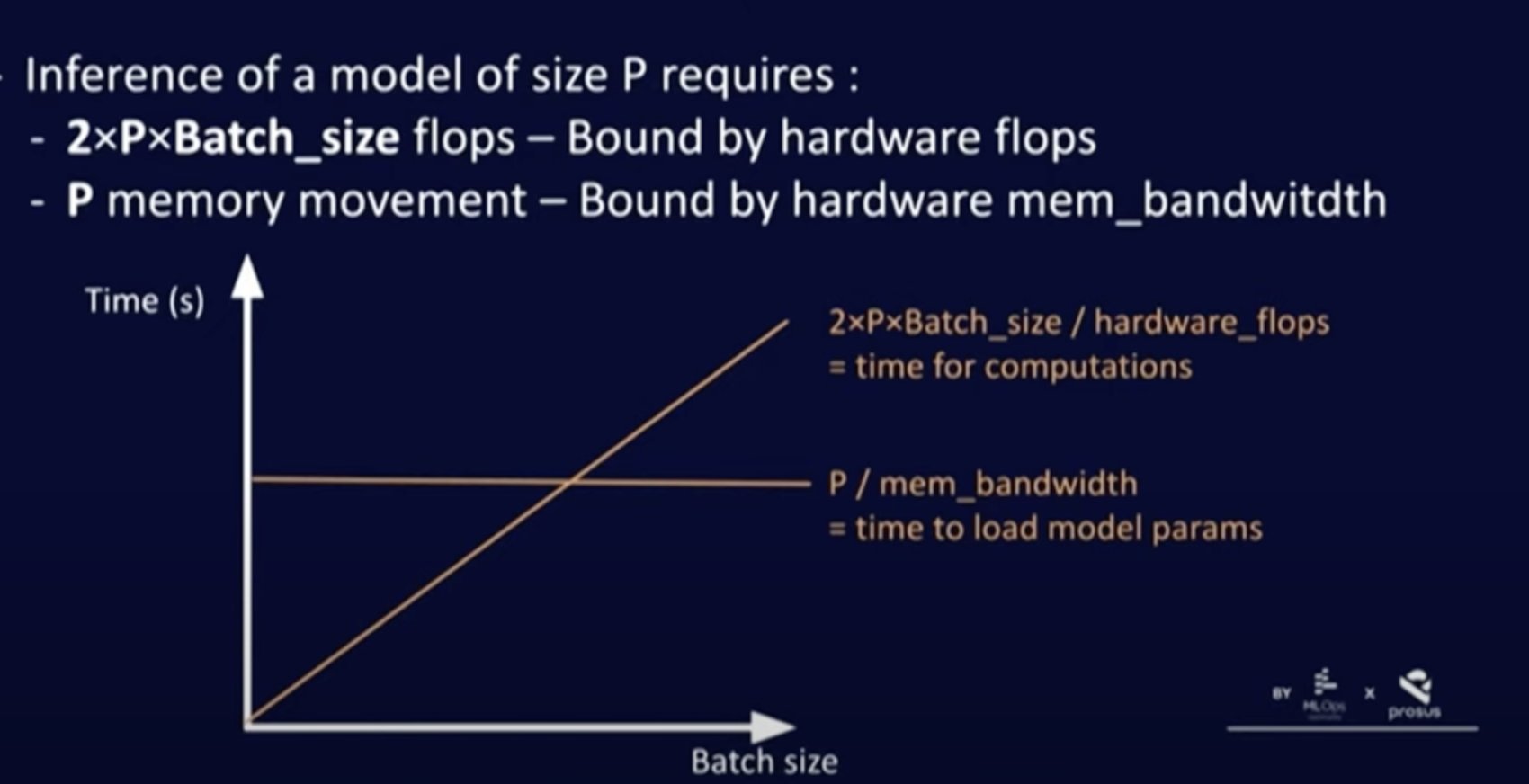
- If we do inference with batch size less than the optimal batch size then we are memory bound (wasting flops). When the batch size is less that means GPU is capable of executing more flops while the model is loading and hence wasting flops.
- When greater batch size is used then we are compute bound (latency increases). This is because when we use a bigger batch size, then the flops required is greater than than the memory bandwidth.
A100-80GB GPU Specs : 2.0TB/sec Memory Bandwidth, 312 TFLOPs (FP16)
H100-80GB GPU Specs : 3.3TB/sec Memory Bandwidth, 395 TFLOPs (FP16)
Batching Strategies
Unlike traditional deep learning models, batching for LLMs can be challenging due to the iterative nature of their inference. These are some llm batching strategies:
Static Batching
In static batching, the batch size remains fixed until the inference process is complete. Even if some requests in the batch finish earlier, no new requests can be added until all the requests in that batch are finished. This can lead to GPU underutilization.
Dynamic Batching
Dynamic batching involves aggregating multiple input requests within a specific time window into a single batch for simultaneous processing, instead of handling each request individually. However, it shares the same limitations as static batching, such as inefficient GPU utilization.
Inflight Batching
Also known as continuous batching or batching with iteration-level scheduling, this approach allows new sequences to be added to the batch as soon as a sequence completes. This results in higher GPU utilization compared to static batching.

Positional Encodings
Positional encodings injects some information about relative/absolute position of the tokens in sequence. Generally absolute position encodings like assigning
a number like 1,2,3 etc as postitional encoding for each time step linearly is not used. The problem with this approach is that not only the values could get quite large, but also our model can face sentences longer than the ones in training. In addition, our model may not see any sample with one specific length which would hurt generalization of our model.
One might think to assign positional encoding in some range like [0,1] where 0 means first and 1 means last time step. One of the problems it will introduce is that you can’t figure out how many words are present within a specific range. In other words, time-step delta doesn’t have consistent meaning across different sentences.
Following are some positional encodings used today :
Sinusoidal Positional Encoding
The positions are encoded using sine and cosine functions of different frequencies, allowing the model to distinguish between different token positions in a sequence. The formula is:
$$ PE_{(pos, 2i)} = \sin \left( \frac{pos}{10000^{\frac{2i}{d}}} \right), \quad PE_{(pos, 2i+1)} = \cos \left( \frac{pos}{10000^{\frac{2i}{d}}} \right) $$
where \( pos \) is the position, \( i \) is the dimension index, and \( d \) is the embedding dimension.
Sinusoidal position embedding approach does not enable transformers to extrapolate to inputs longer than the ones they were trained on.
RoPe
Rotary Positional Encoders (RoPE) introduces a rotational transformation to the embedding vectors, allowing positional information to be encoded in a more flexible way. It rotates the query and key vectors in the attention mechanism based on their relative positions. This approach can handle long sequences more efficiently. The rotation is applied using:
$$ \mathbf{z} = \mathbf{x} \cos(\theta) + \mathbf{x_{\perp}} \sin(\theta) $$
where \( \mathbf{x} \) is the embedding, \( \mathbf{x_{\perp}} \) is a 90-degree shifted version of \( \mathbf{x} \), and \( \theta \) is a function of the token position. RoPE is highly effective in self-attention mechanisms for sequential tasks.
RoPE enables
valuable properties, including the flexibility of sequence length, decaying inter-token dependency
with increasing relative distances, and the capability of equipping the linear self-attention with
relative position encoding
ALiBi
Attention with Linear Biases (ALiBi) does not add positional embeddings to word embeddings. It adds a linear bias to query-key attention scores based on the distance between tokens. The bias penalizes distant tokens more than closer ones, effectively guiding attention to focus more on nearby tokens. Unlike fixed positional encodings, ALiBi introduces a bias term directly into the attention mechanism to handle long-range dependencies without learning explicit position embeddings. The bias is:
$$ \text{bias}(i,j) = -m \cdot |i - j| $$
where \(i\) and \(j\) are the positions of the tokens, and \(m\) is a constant that controls the strength of the bias.
Attention Variations
In large language models (LLMs), attention mechanisms are central to processing and understanding sequences of data (like text). As models get larger and need to handle longer sequences, various specialized attention mechanisms are developed to manage memory, compute, and efficiency. Here’s an explanation of Paged, Flash, Sliding Window, and Grouped Query attention mechanisms:
Paged Attention
PagedAttention partitions the KV cache of each sequence into KV blocks. Each block contains the key and value vectors for a fixed number of tokens,1 which we denote as KV blocksize(𝐵). During the attention computation, the PagedAttention kernel identifies and fetches different KV blocks separately. The PagedAttention algorithm allows the KV blocks to be stored in non-contiguous physical memory, which enables more flexible paged memory management
Flash Attention
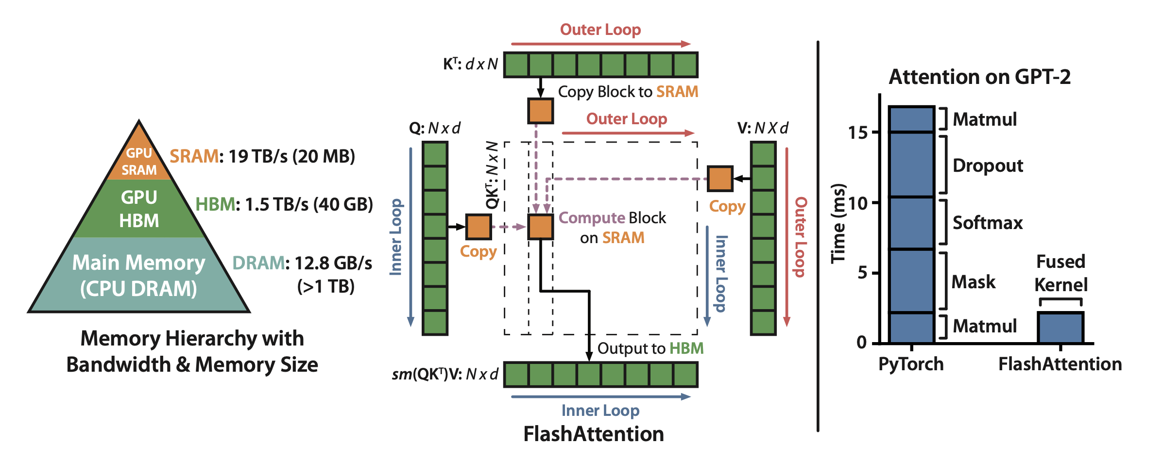
FlashAttention is an IO-aware exact attention algorithm that uses tiling to reduce the number of memory reads/writes between GPU high bandwidth memory (HBM) and GPU on-chip SRAM. FlashAttention uses tiling to prevent materialization of the large 𝑁 × 𝑁 attention matrix (dotted box) on (relatively) slow GPU HBM. In the outer loop (red arrows), FlashAttention loops through blocks of the K and V matrices and loads them to fast on-chip SRAM. In each block, FlashAttention loops over blocks of Q matrix (blue arrows), loading them to SRAM, and writing the output of the attention computation back to HBM. Right: Speedup over the PyTorch implementation of attention on GPT-2. FlashAttention does not read and write the large 𝑁 × 𝑁 attention matrix to HBM, resulting in an 7.6× speedup on the attention computation.
Sliding Window Attention
The number of operations in vanilla attention is quadratic in the sequence length, and the memory increases linearly with the number of tokens. At inference time, this incurs higher latency and smaller throughput due to reduced cache availability. To alleviate this issue, sliding window attention was introduced by Mistral where each token can attend to at most W tokens from the previous layer (here, W = 3). Note that tokens outside the sliding window still influence next word prediction. At each attention layer, information can move forward by W tokens. Hence, after k attention layers, information can move forward by up to k × W tokens.
Grouped Query Attention
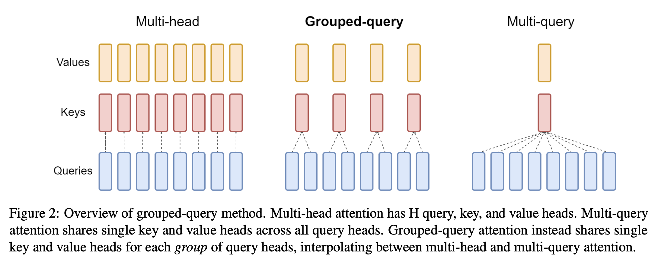
Grouped Query Attention optimizes the attention computation by grouping similar queries together, reducing the number of attention calculations. Grouped Query Attention (GQA) is a method that interpolates between multi-query attention (MQA) and multi-head attention (MHA) in Large Language Models (LLMs). It aims to achieve the quality of MHA while maintaining the speed of MQA.
Quantization
Quantization doesn’t mean truncating/rounding. Quantization reduces the bit-precision of deep learning models which helps to reduce the model size and accelerate inference. Quantization techniques fall into two categories :
Asymmetric Quantization
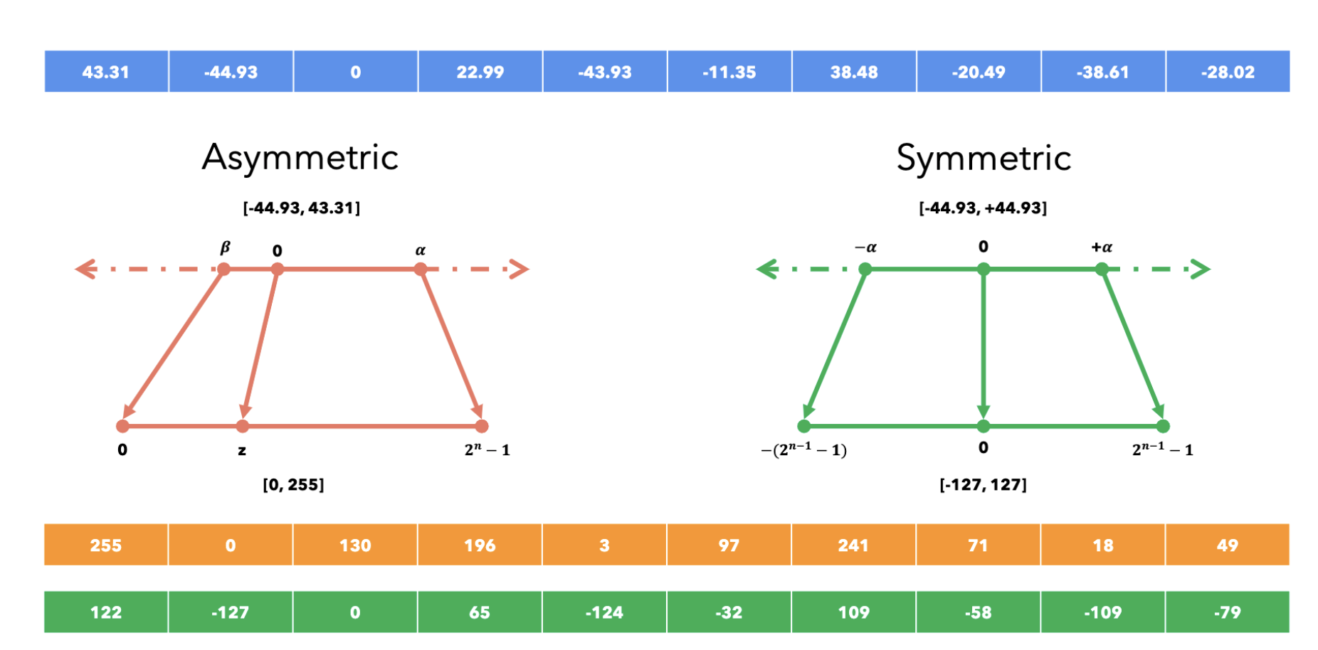
It allows to map a series of floating point numbers in the range \( [\beta, \alpha] \) into another range \( [0, 2^{n}] \). For example, by using 8 bits, we can represent floating-point numbers in the range [0, 255].
Formula for n-bit asymmetric conversion:
\( x_q = clamp(\lfloor \frac{x_f}{s} \rfloor + z;0;2^n - 1 ) \)
Here, \( s= \frac{\alpha - \beta}{2^n -1 } \) and \( z = \lfloor -1*\frac{\beta}{s} \rfloor \)
Dequantize with \( x_f = s(x_q - z) \) . In asymmetric quantization \( \beta \ and \ \alpha \) can be chosen largest and smallest value in the original precision. But it will be sensitive outliers, so these values should be chosen on percentile basis.
Symmetric Quantization
It allows to map a series of floating point numbers in the range \( [-\alpha, \alpha] \) into another range \( [-(2^{n-1} -1), 2^{n-1}-1] \). For example, by using 8 bits, we can represent floating-point numbers in the range [-127, 127].
Formula for n-bit asymmetric conversion:
\( x_q = clamp(\lfloor \frac{x_f}{s} \rfloor ;-(2^{n-1}-1);2^{n-1} - 1 ) \)
Here, \( s= \frac{abs(\alpha)}{2^{n-1} -1 } \)
Dequantize with \( x_f = s*x_q \)
In symmetric quantization \( \alpha \) can be chosen highest absolute value in the original precision. But it will be again sensitive outliers, so these values should be chosen on percentile basis.
Symmetric vs Asymmetric Quantization
A neural network model can be quantized in the following settings :
Post-Training Quantization
If a model needs to be quantized, then we need some sample unlabeled data for calculating the scale (s) and zero (z) parameters which is need for asymmetric quantization. We basically run inference on the model using a few inputs and observe the typical output to calculate the scale (s) and zero (z). This process is called calibration.
Quantization-Aware Training
In this, we insert some fake modules/layers in the computation graph of the model to simulate the effect of the quantization during training. This way, the loss function gets used to update weights that constantly suffer from the effect of quantization.
But there is a problem, as these quantization operations are non-differentiable and it creates a problem while backpropagation. Solution for this is to approximte the gradient with Straight Through Estimator (STE) approximation. The STE approximation results in 1 if the value being quantized is in the range \( [\alpha, \beta] \), otherwise it is 0.
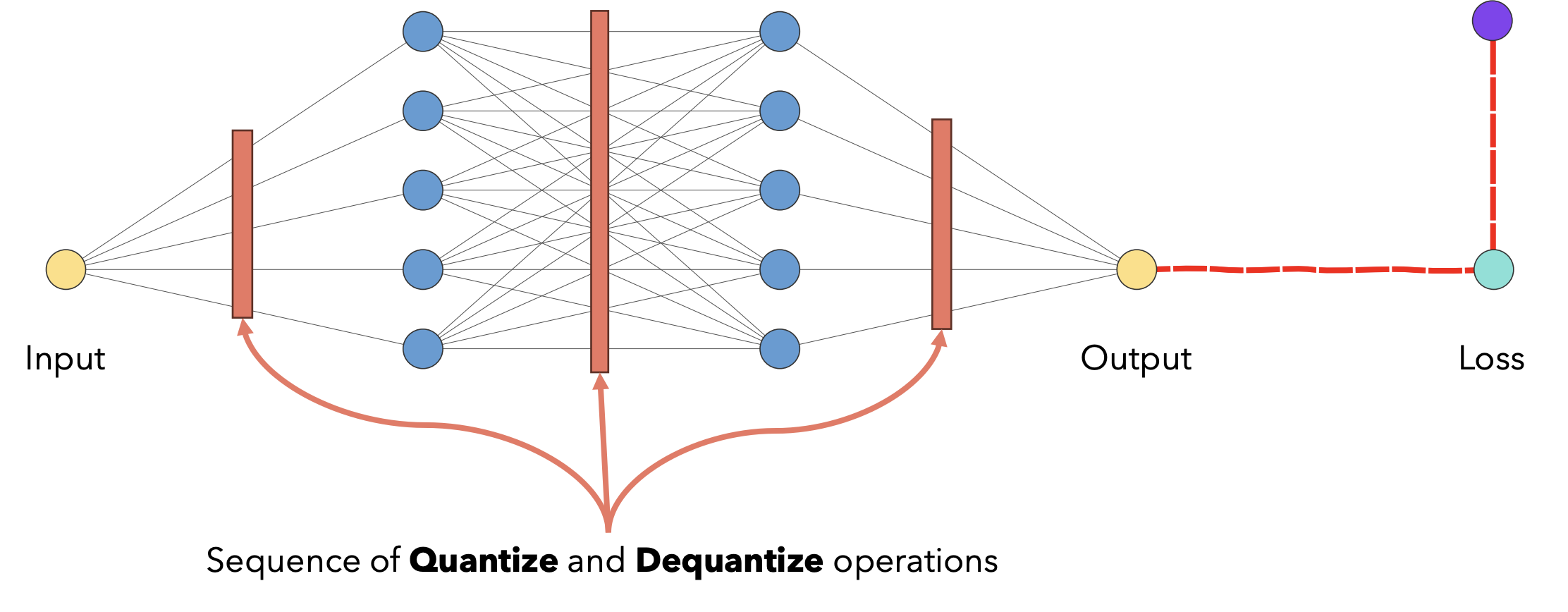
Quantization-Aware Training
Quantization is active area of research now, and these are some more quantization techniques:
Activation-Aware Weight Quantization Not all the weights are equally important for LLM’s performance. There is a small fraction (0.1%-1%) of salient weights; skipping the quantization of these salient weights will significantly reduce the quantization loss.
GPT-Q : GPT-Q focuses on accurate post-training quantization by optimizing the parameters using fewer bits (such as 4-bit integers) while preserving key performance metrics. It leverages a block-wise optimization approach to retain accuracy. This method allows for more efficient deployment of large models in resource-constrained environments, such as edge devices, with minimal loss in performance.
Optimizations Tricks
Model Parallelism
Model Parallelism or Tensor parallelism occurs when each tensor is split up into multiple chunks, and each chunk of the tensor can be placed on a separate GPU. During computation, each chunk gets processed separately in-parallel on different GPUs and the results (final tensor) can be computed by combining results from multiple GPUs, e.g. a 1000×1000 weight matrix would be split into a 1000×250 matrix if you use four GPUs
Pipeline parallelism occurs when a model is split up in-depth and different full layers are placed onto different GPUs/nodes. That is in pipeline parallelism, each GPU hold a fraction of layers. Pipeline parallelism helps distribute the model’s weights across multiple GPUs, but one GPU may remain idle at times. During training, you can pipeline batches through the GPUs (as the first batch moves to the next GPU, a new batch starts on the first GPU). However, this approach doesn’t work efficiently for single-sample requests, although it can still be applied for multiple requests.
Pipeline Parallelism has better communication efficiency as compared to Model Parallelism. A pipeline-parallel model communicates \( d_{model} \) per accelerator, whereas in a model-parallel setup, the communication load is \( N*d_{model} \) per layer, where N is the number of accelerators.
Speculative Decoding
Speculative models speed up inference by predicting multiple tokens at once. This approach involves running two models in parallel: the target model (the main LLM we want to use) and the draft model (a smaller model that helps accelerate inference).
Instead of generating one token at a time, the draft model first predicts a batch of possible next tokens. These tokens are then validated by the larger model, which processes different subsets of the batch in parallel to avoid slowing down the process. If the larger model confirms the predictions, they are accepted, and the process is repeated.
Speculative decoding is highly dependent on the draft model. MEDUSA is an LLM inference acceleration framework with multiple decoding heads. It enhances LLM inference by adding extra decoding heads to predict multiple subsequent tokens in parallel. Using a tree-based attention mechanism, MEDUSA constructs multiple candidate continuations and verifies them simultaneously at each decoding step. By leveraging parallel processing, MEDUSA significantly reduces the number of decoding steps required.
Prefix Caching
Prefix caching is a caching strategy where responses are cached based on the prefix of the request URL or key. Instead of caching an exact match for the entire URL, the cache stores data for a common prefix that multiple requests might share. When a request is made, the system checks if the prefix matches any cached data, and if it does, returns the cached response. This method is particularly useful when dealing with requests that share a common base (e.g., /api/users/), allowing for more efficient reuse of cached content. It helps reduce redundant fetching for similar requests and improves performance.
GEMM Autotuning
GEMM (General Matrix Multiplication) autotuning is an optimization technique that fine-tunes matrix multiplication operations for better performance on specific hardware. Since GEMM is a core operation in deep learning models, autotuning tests various algorithmic configurations, such as tile sizes and memory access patterns, to find the best-performing setup. This tuning process is specific to the hardware’s architecture (e.g., GPUs, CPUs) and maximizes resource utilization, leading to faster and more efficient matrix computations during model training or inference. By reducing computational bottlenecks, GEMM autotuning significantly accelerates performance.
Layer Fusion
Layer fusion in large language model (LLM) inferencing is a technique that combines multiple neural network layers into a single computational step, optimized to run with one kernel. This reduces the need for separate data transfers between layers and increases math density, leading to faster computation. For example, in a multi-head attention block, all operations like matrix multiplications, attention scoring, and projections can be fused into one kernel. This not only accelerates the inference process but also minimizes memory overhead without changing the model’s architecture or outputs.
References
- https://arxiv.org/abs/1706.03762
- https://arxiv.org/abs/2309.06180
- https://arxiv.org/abs/2310.06825
- https://arxiv.org/abs/2305.13245
- https://arxiv.org/abs/2205.14135
- https://kipp.ly/transformer-param-count/
- https://kipp.ly/transformer-inference-arithmetic/
- https://www.anyscale.com/blog/continuous-batching-llm-inference
- https://www.youtube.com/watch?v=0VdNflU08yA&ab_channel=UmarJamil
- https://www.youtube.com/watch?v=mYRqvB1_gRk&ab_channel=MLOps.community
- https://kazemnejad.com/blog/transformer_architecture_positional_encoding/
- https://cerebras.ai/blog/introducing-cerebras-inference-ai-at-instant-speed
- https://developer.nvidia.com/blog/accelerated-inference-for-large-transformer-models-using-nvidia-fastertransformer-and-nvidia-triton-inference-server/